Exercise I-A. Where Uncertainty Enters, and the Fallacy That Follows
Part I. Foundations of GeoAI Risks
Part I. Foundations of GeoAI Risks
Chapters 1, 2 and 3 establish what a GeoAI system is, where uncertainty enters it, and how a foundational vulnerability turns into an operational failure. Chapter 1 develops spatial decision infrastructure and the points at which uncertainty enters, Chapter 2 catalogs the foundational vulnerabilities and shows how they interact, and Chapter 3 works one central case, the apparent rise in natural disasters, and shows that a recorded trend can carry hazard, exposure, vulnerability, observation and classification change at once, which leaves the analyst to separate a change in the world from a change in what observes it.
Two exercises serve this Part. Exercise I-A traces uncertainty through one pipeline and demonstrates the ecological fallacy on real data. Exercise I-B carries Chapter 3's central case, the apparent rise in natural disasters, to the United States tornado record, which the book does not discuss, and separates a change in the world from a change in what was watching it. Instructors with one laboratory session available should assign I-A, which introduces the aggregation ideas that Part II then develops in full.
Fundamentals in play. These exercises use one correlation computed at more than one level of aggregation, the difference between a count and a rate, and normalization by an exposure denominator. Each fails in a known way. A correlation among groups supports no claim about a household, and a rate inherits every defect of its denominator.
| At a glance | |
|---|---|
| Textbook sections | sections 1.4, 1.5, 1.6, 2.2, 2.7, 2.8 |
| Fundamentals covered | inference across levels of aggregation, correlation at group and unit level, uncertainty entry points |
| Technical demand | Tier 1 and Tier 2 required, Tier 3 optional. Python with pandas, numpy and matplotlib |
| Effort | two to three hours including the write up |
| Prerequisites | none |
Overview
Section 1.4 identifies six forms of uncertainty along the GeoAI decision chain, being observation, data, representational, model, interpretive and decision uncertainty. Section 2.2 then works the ecological fallacy, in which a relationship observed among groups gets applied to the individuals inside them. This exercise makes both concrete on one dataset the student can hold in view.
Students trace a single pipeline from a Census survey response through the published estimate, the geographic unit, the derived index and the resulting ranking, tagging what enters at each stage and what the next stage can no longer recover. They then compute one relationship at county level and at block group level and report how far apart the two answers sit. The gap measures the scale effect of section 2.3, and the exercise then asks what claim about a person either figure would support, the question on which the ecological fallacy of section 2.2 turns. Section 2.7 then shows how these vulnerabilities interact, and the exercise closes by asking the student to name one such interaction from their own results.
Step by step
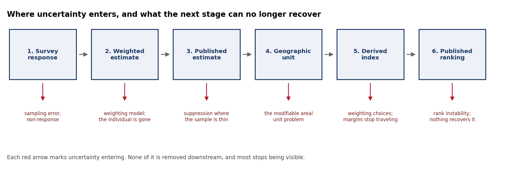
- Trace the pipeline. Tier 1. Change to the toolkit folder inside GeoAI_Exercises and type python exercise_1a.py. The program prints the six stages the Mississippi data passes through, from survey response to published ranking, with what happens and what uncertainty enters at each. Record the six stages and name, for each one, one kind of uncertainty that enters there, the form of uncertainty from section 1.4 it belongs to, and one thing the following stage can no longer recover.
- Measure the scale effect. Tier 1. Record the correlation between poverty and the share of households without a vehicle at county level and at block group level, then state the relationship each supports. Write the sentence a journalist would write from the county figure, then write the sentence the block group figure supports, and state what neither supports about any individual household.
- Find the reversal. Tier 1. The program lists counties in which the relationship among that county's own block groups runs opposite to the between-county relationship. Record how many counties show that reversal and give the county codes of three. Section 3.9 notes that a pattern observed at one scale may disappear or reverse at another, and this step looks for that reversal inside Mississippi counties. State whether any within-county correlation is large enough to distinguish from zero for its number of block groups.
- Change the minimum. Tier 2. Open exercise_1a.py and change
MIN_BGat the top of the file from 8 to 12 and then to 20, rerunning after each change. Record how the number of counties tested and the number of reversals change, and state what that sensitivity says about the reversal count as evidence.
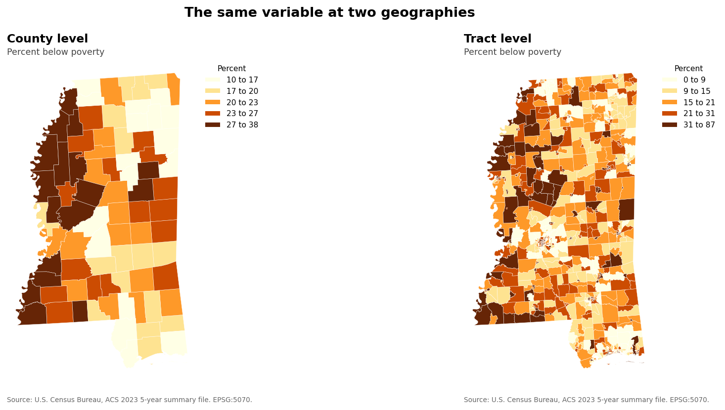
- Map it. Tier 1. The program maps the county level result beside the tract level result. Record both maps and state which one a decision maker would find more persuasive, then state which one is more likely to be right about a household, and explain why those two answers differ.
- Name an interaction. Tier 1. Name one way the scale effect you measured in Step 2 could combine with another foundational vulnerability from section 2.7 in a decision built on these data, and cite the numbers that make it plausible.
- Read the code and complete the handoff. Tier 1. Annotate the block that computes the relationship at each geography and the block that tests each county for a reversal, and answer the questions in the decisions file.
- Ask the assistant. Tier 3, optional, ten points. Give an assistant the county table with the single instruction to describe the relationship between poverty and households without a vehicle in Mississippi, and record whether it warned you about inference to individuals without being asked.