Exercise I-B. Signal, or a Change in What Was Watching
Part I. Foundations of GeoAI Risks
| At a glance | |
|---|---|
| Textbook sections | sections 3.2, 3.3, 3.7, 3.9, 3.11 |
| Fundamentals covered | denominators, exposure normalization, detection regimes, change point reasoning |
| Technical demand | Tier 1 and Tier 2 required. Python with pandas, numpy and matplotlib |
| Effort | three hours including the write up and the reading |
| Prerequisites | none |
Overview
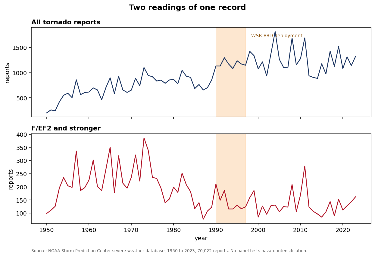
Section 3.2 argues that more data can look like more disasters, and the United States tornado record is the cleanest available demonstration because the observing system changed on a documented schedule. Reports rise steeply across the period of record, the population exposed to being a witness rose across the same period, and a national radar network was deployed through the 1990s. This exercise separates those contributions as far as the data allows and states plainly where separation stops being possible. That last clause is the part students omit, and it is the part a reviewer will test first.
None of the analysis here tests whether hazards have intensified, and the program repeats that statement on screen and in its figure. What it tests is whether a count can be read as a rate, which is a question about denominators and detection, and it applies two of the nine techniques in the Signal-versus-Symptom Analytic Toolkit of section 3.9 (Table 3.9.1), normalization and the detection audit.
Step by step
- Plot the raw count. Tier 1. Change to the toolkit folder inside GeoAI_Exercises and type python exercise_1b.py. Record the annual report totals and describe the trend in one sentence. This is the figure that circulates and the exercise begins there deliberately.
- Restrict to the stronger events. Tier 1. Record annual counts restricted to the higher intensity categories. These depend less on detection, since strong tornadoes usually leave surveyed damage, but they depend on how damage was rated, and the rating scale changed from the Fujita to the Enhanced Fujita scale in 2007. State how the restricted series differs from the raw series.
- Normalize by exposure. Tier 1. The program computes a rate per million residents when a national population series is present in snapshots, and it reports the rate panel as unavailable when none is present. Record the rate where the program reports one. State in either case what a population denominator does and does not control for, and name the population series you would use.
- Mark the detection change. Tier 1. The program marks the radar deployment window on every panel. State whether the raw series changes behavior across that window and whether the intensity restricted series does.
- Move the intensity threshold. Tier 2. Change
STRONGat the top of exercise_1b.py from 2 to 3, rerun, and record how the restricted series and the comparison across the radar window change. State whether the pattern from Step 2 depends on where the threshold sits.
- State the limits. Tier 1. Write one paragraph naming what this analysis cannot determine, and explain why the intensity restricted series is better evidence about the hazard while remaining imperfect evidence.
- Read the code and complete the handoff. Tier 1. Annotate the function that supplies the denominator and answer the decisions file.